Create a Pivot table for Payment Summaries in Excel

Objective

In the tutorials section of this module, you already learned how to create a payment overview, which you can send to your payroll providers. That tutorial covers a simple way of accumulating all the data your payroll provider needs with just a few clicks.

However, if you would like to provide more information and analysis or analyze the payment information in more depth yourself, it makes sense to do so using an excel file, which can be easily created using you HR for Dynamics data.

There are three steps to creating more detailed payment summaries in Excel:

First, you need to create a template for payment summaries in HR for Dynamics and download it.

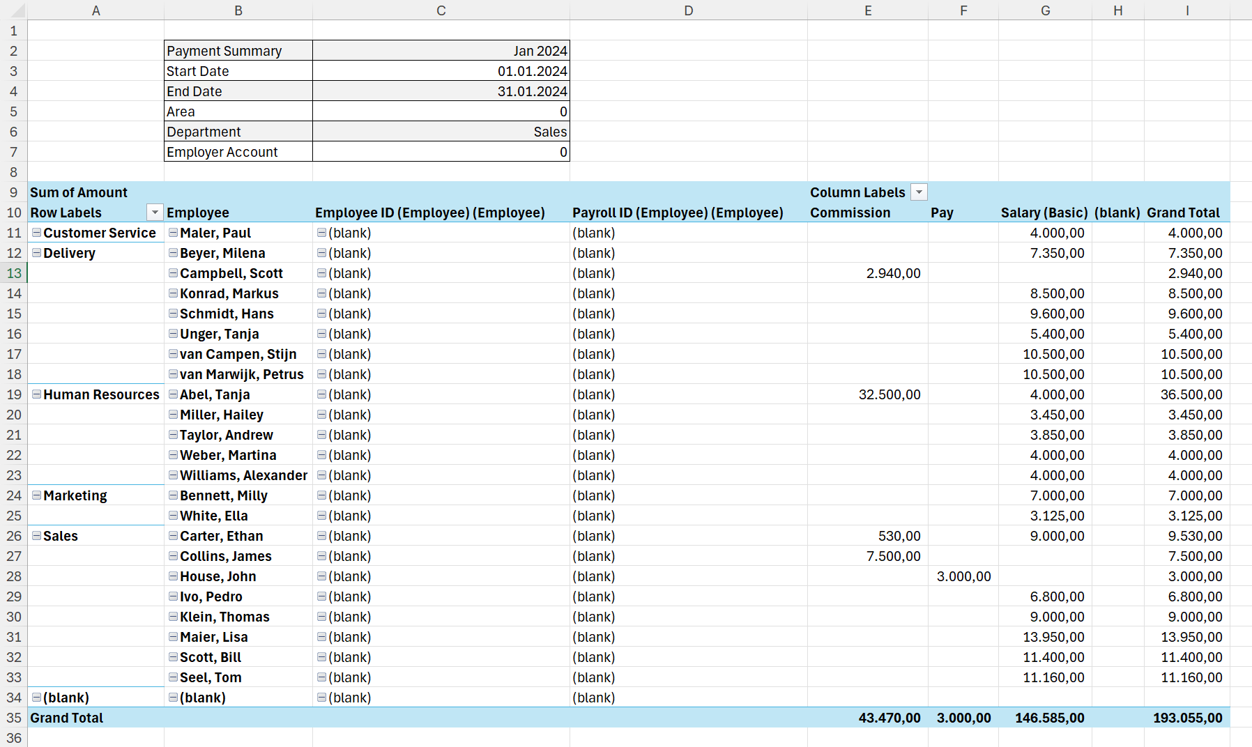
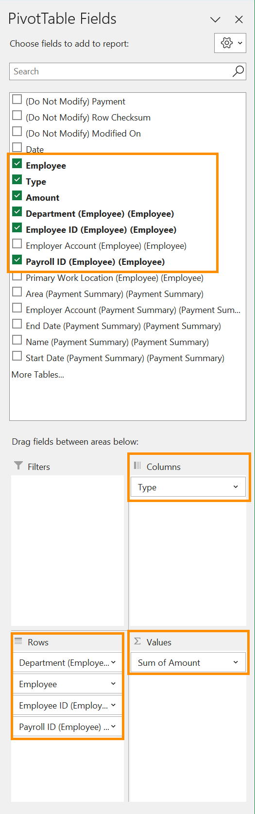
Secondly you need to create a pivot table in your downloaded Excel template to specify the parameters for your analysis. pivot tables can be used to summarize, analyze and visualize large amounts of data. When preparing a document for your payroll provider, you can benefit from the pivot table, ensuring accuracy, compliance, and efficiency in the process. They are easy to use, and provide an easy overview, since they can be linked with charts and graphs. This tutorial covers that second part.

Thirdly, the created Excel file with the pivot table needs to be uploaded back into HR for Dynamics.

From there, you can use the template to analyze every payment summary easily, or send the more detailed payment information to your payroll provider.

Process

HR Manager
Export data to Excel
HR Manager
Create pivot table

Prerequisites

  • The Excel template for payment summaries has already been generated and downloaded

Click Through

  • Open the Excel file you exported
  • On the ribbon enable editing
  • In the ribbon, go to the tab Insert
  • Add Pivot Table
  • Select From Table/Range
  • As Range, add Table1 (if it's not filled automatically yet)
  • Choose New Worksheet for Pivot Table report to be placed
  • Click on OK
  • In the new sheet, we will create the link between employees, departments, and the amount to be received
  • Drag the fields from the top to the areas, according to the following: (Screenshot)
    • Columns: Type
    • Rows: Department, Employee, Employee ID and Payroll ID
    • Values: Amount
  • In the bottom right, click on Sum of Amount and select Value Field Settings
  • Select Sum and click on OK
  • Click on Department and select Field Settings
    • In the ribbon Subtotals & Filters select None
    • In the ribbon Layout & Print select Show item labels in tabular form
    • Click on OK
  • Make the same settings for the rows Employee, Employee ID, and Payroll ID
  • Next, we ensure that the table has the content refreshed every time new data is added:
    • In the Pivot Table, right click on any field and select Pivot Table Options
    • In the tab Data, select Refresh data when opening the file
    • Click on OK
  • Now we create new tables to summarize the content of the Payment Sheet:
  • Above the recently created table, add at least 6 more rows
    • Right click on an empty cell above the table and select Insert - Entire Row - OK
    • Repeat this 5-6 times
  • Inside the new cells, type:
    • Cell B2: Payment Summary
    • Cell B3: Start Date
    • Cell B4: End Date
    • Cell B5: Area
    • Cell B6: Department
    • Cell B7: Employer Account
  • Now we are going to create a formula to connect the two different sheets
    • Click next to Payment Summary (Cell C2) and enter an Equal Sign (=)
    • At the bottom of the page, go to Payment Sheet
    • Click on the second cell of the Name (Payment Summary) - Row
    • Press Enter to confirm the selection
    • Repeat these steps for Start Date, End Date, Area, Department and Employer Account
      • For Start Date, enter the second cell of the Start Date row; for End Date, the second cell of the End Date row, etc.
  • Change to Payment - Sheet
  • Beginning with the second row, mark all rows containing data, right-click and Delete - Entire Row.
    • This is because you don't need the exported data anymore, your template is now blank and ready for future use.
  • Now go to the Pivot Table and click on any field before you save
    • This will ensure that every time you use the template, it will open this sheet
  • Your table is now ready to be used
  • Save and Close the Excel file

Hint

  • The template name in Dynamics will be the same as the file name

Result

Below, you see what such a Pivot table could look like. As a next step, import the template for future use.
Image
HR